
Blog
2020-02-17
This is the sixth post in a series of posts about my PhD thesis.
Before we move on to some concluding remarks and notes about possible future work,
I must take this opportunity to thank my co-supervisors Timo Betcke and Erik Burman,
as without their help, support, and patience, this work would never have happened.
Future work
There are of course many things related to the work in my thesis that could be worked on in the future by me or others.
In the thesis, we presented the analysis of the weak imposition of Dirichlet, Neumann, mixed Dirichlet–Neumann, Robin, and Signorini boundary conditions on Laplace's equation;
and Dirichlet, and mixed Dirichlet–Neumann conditions on the Helmholtz equation. One area of future work would be to extend this analysis to other conditions, such as the imposition of
Robin conditions on the Helmholtz equation. It would also be of great interest to extend the method to other problems, such as Maxwell's equations. For Maxwell's equations, it looks like the
analysis will be significantly more difficult.
In the problems in later chapters, in particular chapter 4, the ill-conditioning of the matrices obtained from the method led to slow or even inaccurate solutions.
It would be interesting to look into alternative preconditioning methods for these problems as a way to improve the conditioning of these matrices. Developing these preconditioners appears to be
very important for Maxwell's equations: general the matrices involved when solving Maxwell's equations tend to be very badly ill-conditioned, and in the few experiments I ran to try out
the weak imposition of boundary conditions on Maxwell's equations, I was unable to get a good solution due to this.
Your work
If you are a undergraduate or master's student and are interested in working on similar stuff to me, then you could look into
doing a PhD with Timo and/or Erik (my supervisors).
There are also many other people around working on similar stuff, including:
- Iain Smears, David Hewett, and others in the Department of Mathematics at UCL;
- Garth Wells in the Department of Engineering at Cambridge;
- Patrick Farrell, Carolina Urzua-Torres, and others in the Department of Mathematics at Oxford;
- Euan Spence, Ivan Graham, and others in the Department of Mathematics at Bath;
- Stéphanie Chaillat-Loseille, and others at ENSTA in Paris;
- Marie Rognes, and others at Simula in Oslo.
There are of course many, many more people working on this, and this list is in no way exhaustive. But hopefully this list can be a useful starting point for anyone interested in studying this area
of maths.
Previous post in series
This is the sixth post in a series of posts about my PhD thesis.
(Click on one of these icons to react to this blog post)
You might also enjoy...

Comments
Comments in green were written by me. Comments in blue were not written by me.
Add a Comment
2020-02-16
This is the fifth post in a series of posts about my PhD thesis.
In the fifth and final chapter of my thesis, we look at how boundary conditions can be weakly imposed on the Helmholtz equation.
Analysis
As in chapter 4, we must adapt the analysis of chapter 3 to apply to Helmholtz problems. The boundary operators for the Helmholtz equation satisfy less strong
conditions than the operators for Laplace's equation (for Laplace's equation, the operators satisfy a condition called coercivity; for Helmholtz, the operators
satisfy a weaker condition called Gårding's inequality), making proving results about Helmholtz problem harder.
After some work, we are able to prove an a priori error bound (with \(a=\tfrac32\) for the spaces we use):
$$\left\|u-u_h\right\|\leqslant ch^{a}\left\|u\right\|$$
Numerical results
As in the previous chapters, we use Bempp to show that computations with this method match the theory.
)
The error of our approximate solutions of a Dirichlet (left) and mixed Dirichlet–Neumann problems in the exterior of a sphere with
meshes with different values of \(h\). The dashed lines show order \(\tfrac32\) convergence.
Wave scattering
Boundary element methods are often used to solve Helmholtz wave scattering problems. These are problems in which a sound wave is travelling though a medium (eg the air),
then hits an object: you want to know what the sound wave that scatters off the object looks like.
If there are multiple objects that the wave is scattering off, the boundary element method formulation can get quite complicated. When using weak imposition,
the formulation is simpler: this one advantage of this method.
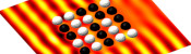
The following diagram shows a sound wave scattering off a mixure of sound-hard and sound-soft spheres.
Sound-hard objects reflect sound well, while sound-soft objects absorb it well.
)
A sound wave scattering off a mixture of sound-hard (white) and sound-soft (black) spheres.
If you are trying to design something with particular properties—for example, a barrier that absorbs sound—you may want to solve
lots of wave scattering problems on an object on some objects with various values taken for their reflective properties. This type of problem is often called an inverse problem.
For this type of problem, weakly imposing boundary conditions has advantages: the discretisation of the Calderón projector can be reused for each problem, and only the terms
due to the weakly imposed boundary conditions need to be recalculated. This is an advantages as the boundary condition terms are much less expensive (ie they use much less time and memory)
to calculate than the Calderón term that is reused.
This concludes chapter 5, the final chapter of my thesis.
Why not celebrate reaching the end by cracking open the following figure before reading the concluding blog post.
)
An acoustic wave scattering off a sound-hard champagne bottle and a sound-soft cork.
Previous post in series
This is the fifth post in a series of posts about my PhD thesis.
Next post in series

(Click on one of these icons to react to this blog post)
You might also enjoy...
Comments
Comments in green were written by me. Comments in blue were not written by me.
Add a Comment
2020-02-13
This is the fourth post in a series of posts about my PhD thesis.
The fourth chapter of my thesis looks at weakly imposing Signorini boundary conditions on the boundary element method.
Signorini conditions
Signorini boundary conditions are composed of the following three conditions on the boundary:
\begin{align*}
u &\leqslant g\\
\frac{\partial u}{\partial n} &\leqslant \psi\\
\left(\frac{\partial u}{\partial n} -\psi\right)(u-g) &=0
\end{align*}
In these equations, \(u\) is the solution, \(\frac{\partial u}{\partial n}\) is the derivative of the solution in the direction normal to the boundary, and
\(g\) and \(\psi\) are (known) functions.
These conditions model an object that is coming into contact with a surface: imagine an object that is being pushed upwards towards a surface. \(u\) is the height of the object at
each point; \(\frac{\partial u}{\partial n}\) is the speed the object is moving upwards at each point; \(g\) is the height of the surface; and \(\psi\) is the speed at which the upwards force will cause
the object to move. We now consider the meaning of each of the three conditions.
The first condition (\(u \leqslant g\) says the the height of the object is less than or equal to the height of the surface. Or in other words, no part of the object has been pushed through
the surface. If you've ever picked up a real object, you will see that this is sensible.
The second condition (\(\frac{\partial u}{\partial n} \leqslant \psi\)) says that the speed of the object is less than or equal to the speed that the upwards force will cause. Or in other words,
the is no extra hidden force that could cause the object to move faster.
The final condition (\(\left(\frac{\partial u}{\partial n} -\psi\right)(u-g)=0\)) says that either \(u=g\) or \(\frac{\partial u}{\partial n}=\psi\). Or in other words, either the object is touching
the surface, or it is not and so it is travelling at the speed caused by the force.
Non-linear problems
It is possible to rewrite these conditions as the following, where \(c\) is any positive constant:
$$u-g=\left[u-g + c\left(\frac{\partial u}{\partial n}-\psi\right)\right]_-$$
The term \(\left[a\right]_-\) is equal to \(a\) if \(a\) is negative or 0 if \(a\) is positive (ie \(\left[a\right]_-=\min(0,a)\)).
If you think about what this will be equal to if \(u=g\), \(u\lt g\), \(\frac{\partial u}{\partial n}=\psi\), and \(\frac{\partial u}{\partial n}\lt\psi\), you can convince yourself
that it is equivalent to the three Signorini conditions.
Writing the condition like this is helpful, as this can easily be added into the matrix system due to the boundary element method to weakly impose it. There is, however, a complication:
due to the \([\cdot]_-\) operator, the term we add on is non-linear and cannot be represented as a matrix. We therefore need to do a little more than simply use our favourite
matrix solver to solve this problem.
To solve this non-linear system, we use an iterative approach: first make a guess at what the solution might be (eg guess that \(u=0\)). We then use this guess to calculate the value
of the non-linear term, then solve the linear system obtained when the value is substituted in. This gives us a second guess of the solution: we can do follow the same approach to obtain a third
guess. And a fourth. And a fifth. We continue until one of our guesses is very close to the following guess, and we have an approximation of the solution.
Analysis
After deriving formulations for weakly imposed Signorini conditions on the boundary element method, we proceed as we did in chapter 3 and analyse the method.
The analysis in chapter 4 differs from that in chapter 3 as the system in this chapter is non-linear. The final result, however, closely resembles the results in chapter 3: we obtain
and a priori error bounds:
$$\left\|u-u_h\right\|\leqslant ch^{a}\left\|u\right\|$$
As in chapter 3, The value of the constant \(a\) for the spaces we use is \(\tfrac32\).
Numerical results
As in chapter 3, we used Bempp to run some numerical experiments to demonstrate the performance of this method.
)
The error of our approximate solutions of a Signorini problem on the interior of a sphere with meshes with different values of \(h\) for two choices of combinations of discrete spaces. The
dashed lines show order \(\tfrac32\) convergence.
These results are for two different combinations of the discrete spaces we looked at in chapter 2. The plot on the left shows the expected
order \(\tfrac32\). The plot on the right, however, shows a lower convergence than our a priori error bound predicted. This is due to the matrices obtained when using this combination of spaces
being ill-conditioned, and so our solver struggles to find a good solution. This ill-conditioning is worse for smaller values of \(h\), which is
why the plot starts at around the expected order of convergence, but then the convergence tails off.
These results conclude chapter 4 of my thesis.
Why not take a break and snack on the following figure before reading on.
)
The solution of a mixed Dirichlet–Signorini problem on the interior of an apple, solved using weakly imposed boundary conditions.
Previous post in series
This is the fourth post in a series of posts about my PhD thesis.
Next post in series
(Click on one of these icons to react to this blog post)
You might also enjoy...
Comments
Comments in green were written by me. Comments in blue were not written by me.
Add a Comment
2020-02-11
This is the third post in a series of posts about my PhD thesis.
In the third chapter of my thesis, we look at how boundary conditions can be weakly imposed when using the boundary element method.
Weak imposition of boundary condition is a fairly popular approach when using the finite element method, but our application of it to the boundary element method, and our analysis of
it, is new.
But before we can look at this, we must first look at what boundary conditions are and what weak imposition means.
Boundary conditions
A boundary condition comes alongside the PDE as part of the problem we are trying to solve. As the name suggests, it is a condition on the boundary: it tells us what the
solution to the problem will do at the edge of the region we are solving the problem in. For example, if we are solving a problem involving sound waves hitting an object, the
boundary condition could tell us that the object reflects all the sound, or absorbs all the sound, or does something inbetween these two.
The most commonly used boundary conditions are Dirichlet conditions, Neumann conditions and Robin conditions.
Dirichlet conditions say that the solution has a certain value on the boundary;
Neumann conditions say that derivative of the solution has a certain value on the boundary;
Robin conditions say that the solution at its derivate are in some way related to each other (eg one is two times the other).
Imposing boundary conditions
Without boundary conditions, the PDE will have many solutions. This is analagous to the following matrix problem, or the equivalent system of simultaneous equations.
\begin{align*}
\begin{bmatrix}
1&2&0\\
3&1&1\\
4&3&1
\end{bmatrix}\mathbf{x}
&=
\begin{pmatrix}
3\\4\\7
\end{pmatrix}
&&\text{or}&
\begin{array}{3}
&1x+2y+0z=3\\
&3x+1y+1z=4\\
&4x+3y+1z=7
\end{array}
\end{align*}
This system has an infinite number of solutions: for any number \(a\), \(x=a\), \(y=\tfrac12(3-a)\), \(z=4-\tfrac52a-\tfrac32\) is a solution.
A boundary condition is analagous to adding an extra condition to give this system a unique solution, for example \(x=a=1\). The usual way of imposing
a boundary condition is to substitute the condition into our equations. In this example we would get:
\begin{align*}
\begin{bmatrix}
2&0\\
1&1\\
3&1
\end{bmatrix}\mathbf{y}
&=
\begin{pmatrix}
2\\1\\3
\end{pmatrix}
&&\text{or}&
\begin{array}{3}
&2y+0z=2\\
&1y+1z=1\\
&3y+1z=3
\end{array}
\end{align*}
We can then remove one of these equations to leave a square, invertible matrix. For example, dropping the middle equation gives:
\begin{align*}
\begin{bmatrix}
2&0\\
3&1
\end{bmatrix}\mathbf{y}
&=
\begin{pmatrix}
2\\3
\end{pmatrix}
&&\text{or}&
\begin{array}{3}
&2y+0z=2\\
&3y+1z=3
\end{array}
\end{align*}
This problem now has one unique solution (\(y=1\), \(z=0\)).
Weakly imposing boundary conditions
To weakly impose a boundary conditions, a different approach is taken: instead of substituting (for example) \(x=1\) into our system, we add \(x\) to one side of an equation
and we add \(1\) to the other side. Doing this to the first equation gives:
\begin{align*}
\begin{bmatrix}
2&2&0\\
3&1&1\\
4&3&1
\end{bmatrix}\mathbf{x}
&=
\begin{pmatrix}
4\\4\\7
\end{pmatrix}
&&\text{or}&
\begin{array}{3}
&2x+2y+0z=4\\
&3x+1y+1z=4\\
&4x+3y+1z=7
\end{array}
\end{align*}
This system now has one unique solution (\(x=1\), \(y=1\), \(z=0\)).
In this example, weakly imposing the boundary condition seems worse than substituting, as it leads to a larger problem which will take longer to solve.
This is true, but if you had a more complicated condition (eg \(\sin x=0.5\) or \(\max(x,y)=2\)), it is not always possible to write the condition in a nice way that can be substituted in,
but it is easy to weakly impose the condition (although the result will not always be a linear matrix system, but more on that in chapter 4).
Analysis
In the third chapter of my thesis, we wrote out the derivations of formulations of the weak imposition of Dirichet, Neumann, mixed Dirichlet–Neumann, and Robin conditions on Laplace's equation:
we limited our work in this chapter to Laplace's equation as it is easier to analyse than the Helmholtz equation.
Once the formulations were derived, we proved some results about them: the main result that this analysis leads to is the proof of a priori error bounds.
An a priori error bound tells you how big the difference between your approximation and the actual solution will be.
These bounds are called a priori as they can be calculated before you solve the problem (as opposed to a posteriori error bounds that are calculated after solving the problem
to give you an idea of how accurate you are and which parts of the solution are more or less accurate).
Proving these bounds is important, as proving this kind of bound shows that your method will give a good approximation of the actual solution.
A priori error bounds look like this:
$$\left\|u-u_h\right\|\leqslant ch^{a}\left\|u\right\|$$
In this equation, \(u\) is the solution of the actual PDE problem; \(u_h\) is our appoximation; the \(h\) that appears in \(u_h\) and on the right-hand size is
the length of the longest edge in the mesh we are using; and \(c\) and \(a\) are positive constants. The vertical lines \(\|\cdot\|\) are a measurement of the size of a function.
Overall, the equation says that the size of the difference between the solution and our approximation (ie the error) is smaller than a constant times \(h^a\) times the size of
the solution. Because \(a\) is positive, \(h^a\) gets smaller as \(h\) get smaller, and so if we make the triangles in our mesh smaller (and so have more of them), we will see our error getting
smaller.
The value of the constant \(a\) depends on the choices of discretisation spaces used: using the spaces in the previous chapter gives \(a\) equal to \(\tfrac32\).
Numerical results
Using Bempp, we approximated the solution on a series of meshes with different values of \(h\) to check that we do indeed get order \(\tfrac32\) convergence.
By plotting \(\log\left(\left\|u-u_h\right\|\right)\) against \(\log h\), we obtain a graph with gradient \(a\) and can easily compare this gradient to a gradient of \(\tfrac32\).
Here are a couple of our results:
)
The errors of a Dirichlet problem on a cube (left) and a Robin problem on a sphere (right) as \(h\) is decreased. The dashed lines show order \(\tfrac32\) convergence.
Note that the \(\log h\) axis is reversed, as I find these plots easier to interpret this way found. Pleasingly, in these numerical experiments, the order of convergence agrees with
the a priori bounds that we proved in this chapter.
These results conclude chapter 3 of my thesis.
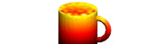
Why not take a break and refill the following figure with hot liquid before reading on.
)
The solution of a mixed Dirichlet–Neumann problem on the interior of a mug, solved using weakly imposed boundary conditions.
Previous post in series
This is the third post in a series of posts about my PhD thesis.
Next post in series
(Click on one of these icons to react to this blog post)
You might also enjoy...
Comments
Comments in green were written by me. Comments in blue were not written by me.
Add a Comment
2020-02-04
This is the second post in a series of posts about my PhD thesis.
During my PhD, I spent a lot of time working on the open source boundary element method Python library Bempp.
The second chapter of my thesis looks at this software, and some of the work we did to improve its performance and to make solving problems with it more simple,
in more detail.
Discrete spaces
We begin by looking at the definitions of the discrete function spaces that we will use when performing discretisation. Imagine that the boundary of our region has been split into a mesh of triangles.
(The pictures in this post show a flat mesh of triangles, although in reality this mesh will usually be curved.)
We define the discrete spaces by defining a basis function of the space. The discrete space will have one of these basis functions for each triangle, for each edge, or for each vertex (or a combination
of these) and the space is defined to contain all the sums of multiples of these basis functions.
The first space we define is DP0 (discontinuous polynomials of degree 0). A basis function of this space has the value 1 inside one triangle, and has the value 0 elsewhere; it
looks like this:
)
Next we define the P1 (continuous polynomials of degree 1) space. A basis function of this space has the value 1 at one vertex in the mesh, 0 at every other vertex, and is linear inside
each triangle; it looks like this:
)
Higher degree polynomial spaces can be defined, but we do not use them here.
For Maxwell's equations, we need different basis functions, as the unknowns are vector functions. The two most commonly spaces are RT (Raviart–Thomas) and NC (Nédélec) spaces.
Example basis functions of these spaces look like this:
)
RT (left) and NC (right) basis functions.
Preconditioning
Suppose we are trying to solve \(\mathbf{A}\mathbf{x}=\mathbf{b}\), where \(\mathbf{A}\) is a matrix, \(\mathbf{b}\) is a (known) vector, and \(\mathbf{x}\) is the vector we are trying to find.
When \(\mathbf{A}\) is a very large matrix, it is common to only solve this approximately, and many methods are known that can achieve
good approximations of the solution. To get a good idea of how quickly these methods will work, we can calculate the condition number of the matrix: the condition number
is a value that is big when the matrix will be slow to solve (we call the matrix ill-conditioned); and is small when the matrix will be fast to solve (we call the matrix well-conditioned).
The matrices we get when using the boundary element method are often ill-conditioned. To speed up the solving process, it is common to use preconditioning: instead of solving \(\mathbf{A}\mathbf{x}=\mathbf{b}\), we can
instead pick a matrix \(\mathbf{P}\) and solve $$\mathbf{P}\mathbf{A}\mathbf{x}=\mathbf{P}\mathbf{b}.$$ If we choose the matrix \(\mathbf{P}\) carefully, we can obtain a matrix
\(\mathbf{P}\mathbf{A}\) that has a lower condition number than \(\mathbf{A}\), so this new system could
be quicker to solve.
When using the boundary element method, it is common to use properties of the Calderón projector to work out some good preconditioners.
For example, the single layer operator \(\mathsf{V}\) when discretised is often ill-conditioned, but the product of it and the hypersingular operator \(\mathsf{W}\mathsf{V}\) is often
better conditioned. This type of preconditioning is called operator preconditioning or Calderón preconditioning.
If the product \(\mathsf{W}\mathsf{V}\) is discretised, the result is $$\mathbf{W}\mathbf{M}^{-1}\mathbf{V},$$ where \(\mathbf{W}\) and \(\mathbf{V}\)
are discretisations of \(\mathsf{W}\) and \(\mathsf{V}\), and \(\mathbf{M}\) is a matrix
called the mass matrix that depends on the discretisation spaces used to discretise \(\mathsf{W}\) and \(\mathsf{V}\).
In our software Bempp, the mass matrices \(\mathbf{M}\) are automatically included in product like this, which makes using preconditioning like this easier to program.
As an alternative to operator preconditioning, a method called mass matrix preconditioning is often used: this method uses the inverse mass matrix \(\mathbf{M}^{-1}\) as a preconditioner (so is like the operator
preconditioning example without the \(\mathbf{W}\)).
More discrete spaces
As the inverse mass matrix \(\mathbf{M}^{-1}\) appears everywhere in the preconditioning methods we would like to use, it would be great if this matrix was well-conditioned: as if it is, it's inverse
can be very quickly and accurately approximated.
There is a condition called the inf-sup condition: if the inf-sup condition holds for the discretisation spaces used, then the mass matrix will be well-conditioned. Unfortunately, the inf-sup
condition does not hold when using a combination of DP0 and P1 spaces.
All is not lost, however, as there are spaces we can use that do satisfy the inf-sup condition. We call these DUAL0 and DUAL1, and they form inf-sup stable pairs with P1 and DP0 (respectively).
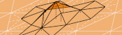
They are defined using the barycentric dual mesh: this mesh is defined by joining each point in a triangle with the midpoint of the opposite side, then making polygons with all the small triangles that
touch a vertex in the original mesh:
)
The mesh (left), the barycentric refinement (centre), and the dual grid (right)
Example DUAL1 and DUAL0 basis functions look like this:
)
DUAL1 (left) and DUAL0 (right) basis functions.
For Maxwell's equations, we define BC (Buffa–Christiansen) and RBC (rotated BC) functions to make inf-sup stable spaces pairs. Example BC and RBC basis functions look like this:
)
Example BC (left) and RBC (right) basis functions.
My thesis then gives some example Python scripts that show how these spaces can be used in Bempp to solve some example problems, concluding chapter 2 of my thesis.
Why not take a break and have a slice of the following figure before reading on.
)
An electromagnetic wave scattering off a perfectly conducting metal cake. This solution was found using a Calderón preconditioned boundary element method.
Previous post in series

This is the second post in a series of posts about my PhD thesis.
Next post in series
(Click on one of these icons to react to this blog post)
You might also enjoy...
Comments
Comments in green were written by me. Comments in blue were not written by me.
Add a Comment