
Blog
2020-01-31
This is the first post in a series of posts about my PhD thesis.
Yesterday, I handed in the final version of my PhD thesis. This is the first in a series of blog posts in which I will attempt to explain what my thesis says with minimal
mathematical terminology and notation.
The aim of these posts is to give a more general audience some idea of what my research is about. If you are looking to build on my work, I recommend that you read
my thesis, or my papers based on parts of it for the full mathematical detail. You may find these posts helpful
with developing a more intuitive understanding of some of the results in these.
In this post, we start at the beginning and look at what is contained in chapter 1 of my thesis.
Introduction
In general, my work looks at using discretisation to approximately solve partial differential equations (PDEs). We primarily focus on three PDEs:
| Laplace's equation | \(-\Delta u=0\) |
If \(u\) represents the temperature in a region,
the region contains no heat sources, and the heat distribution in the region is not changing, then \(u\) a solution of Laplace's equation.
Because of this application, Laplace's equation is sometimes called the steady-state heat equation.
| The Helmholtz equation | \(-\Delta u-k^2u=0\) |
The Helmholtz equation models acoustic waves travelling through a medium.
The unknown \(u\) represents the amplitude of the wave at each point.
The equation features the wavenumber \(k\), which gives the number of waves per unit distance.
| Maxwell's equations | \(\nabla\times\nabla\times e-k^2e=0\) |
Maxwell's equations describe the behaviour of electromagnetic waves. The unknown \(e\) in Maxwell's equatons is an unknown vector, whereas the unknown \(u\) in Laplace and Helmholtz is a scalar.
This adds some difficulty when working with Maxwell's equations.
Discretisation
In many situations, no method for finding the exact solution to these equations is known. It is therefore very important to be able to get accurate approximations of the
solutions of these equations. My PhD thesis focusses on how these can be approximately solved using discretisation.
Each of the PDEs that we want to solve describes a function that has a value at every point in a 3D space: there are an (uncountably) infinite number of points, so these
equations effectively have an infinite number of unknown values that we want to know. The aim of discretisation is to reduce the number of unknowns to a finite number in such a way that
solving the finite problem gives a good approximation of the true solution. The finite problem can then be solved using your favourite matrix method.
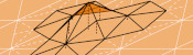
For example, we could split a 2D shape into lots of small triangles, or split a 3D shape into lots of small tetrahedra. We could then try to approximate our solution with a constant inside
each triangle or tetrahedron. Or we could approximate by taking a value at each vertex of the triangles or tetrahedra, and a linear function inside shape. Or we could use quadratic functions or higher
polynomials to approximate the solution. This is the approach taken by a method called the finite element method.
My thesis, however, focusses on the boundary element method, a method that is closely related to the finite element method. Imagine that we want to solve a PDE problem inside a sphere.
For some PDEs (such as the three above), it is possible to represent the solution in terms of some functions on the surface of the sphere. We can then approximate the solution to the problem
by approximating these functions on the surface: we then only have to discretise the surface and not the whole of the inside of the sphere. This method will also work for other 3D shapes, and isn't
limited to spheres.
One big advantage of this method is that it can also be used if we want to solve a problem in the (infinte) region outside an object, as even if the region is infinite, the surface of the object
will be finite. The finite element method has difficulties here, as splitting the infinite region in tetrahedra would require an infinite number of tetrahedra, which destroys the point of discretisation
(although this kind of problem can be solved using finite elements if you split into tetrahedra far enough outwards, then use some tricks where your tetrahedron stop). The finite element method, on the
other hand, works for a much wider range of PDEs, so in many situations it would be the only of these two methods that can be used.
We focus on the boundary element method as when it can be used, it can be a very powerful method.
Sobolev spaces
Much of the first chapter of my thesis looks at the definitions of Sobolev function spaces: these spaces describe the types of functions that we will look for to solve our PDEs.
It is important to frame the problems using Sobolev spaces, as properties of these spaces are used heavily when proving results about our approximations.
The definitions of these spaces are too technical to include here, but the spaces can be thought of as a way to require certain things of the solutions to our problems.
We start be demanding that the function be square integrable: they can be squared the integrated to give a finite answer. Other spaces are then defined by demanding that a
function can be differentiated to give a square integrable derivative; or it can be differentiated twice or more times.
Boundary element method
We now look at how the boundary element method works in more detail. The "boundary" in the name refers to the surface of the object or region that we are solving problems in.
In order to be able to use the boundary element method, we need to know the Green's function of the PDE in question.
(This is what limits the number of problems that the boundary element method can be used to solve.)
The Green's function is the solution as every point in 3D (or 2D if you prefer) except for one point, where it has an infinite value, but a very special type of infinite value.
The Green's function gives the field due to a unit point source at the chosen point.
If a region contains no sources, then the solution inside that region can be represented by adding up point sources at every point on the boundary (or in other words, integrating the Green's function
times a weighting function, as the limit of adding up these at lots of points is an integral). The solution could instead be represented by doing the same thing with the derivative of the Green's function.
We define two potential operators—the single layer potential \(\mathcal{V}\) and the double layer potential \(\mathcal{K}\)—to be the two operators representing the two boundary integrals:
these operators can be applied to weight functions on the boundary to give solutions to the PDE in the region. Using these operators, we write a representation formula that tells us how
to compute the solution inside the region once we know the weight functions on the boundary.
By looking at the values of these potential operators on the surface, and derivative of these values, (and integrating these over the boundary) we can define four boundary operators:
the single layer operator \(\mathsf{V}\),
the double layer operator \(\mathsf{K}\),
the adjoint double layer operator \(\mathsf{K}'\),
the hypersingular operator \(\mathsf{W}\).
We use these operators to write the boundary integral equation that we derive from the representation formula. It is this boundary integral equation that we will apply discretisation
to to find an approximation of the weight functions; we can then use the representation formula to find the solution to the PDE.
The Calderón projector
Using the four boundary operators, we can define the Calderón projector, \(\mathsf{C}\):
$$\mathsf{C}=\begin{bmatrix}
\tfrac12-\mathsf{K}&\mathsf{V}\\
\mathsf{W}&\tfrac12+\mathsf{K}'
\end{bmatrix}$$
This is the Calderón projector for problems in a finite interior region. For exterior problems, the exterior Cadleró is used. This is given by
$$\mathsf{C}=\begin{bmatrix}
\tfrac12+\mathsf{K}&-\mathsf{V}\\
-\mathsf{W}&\tfrac12-\mathsf{K}'
\end{bmatrix}.$$
We treat the Calderón operator like a matrix, even though its entries are operators not numbers. The Calderón projector has some very useful properties that
are commonly used when using the boundary element method. These include:
- \(\mathsf{C}^2=\mathsf{C}\).
- If we apply \(\mathsf{C}\) to a solution of the PDE, the Calderón projector does nothing to the input.
- If we apply \(\mathsf{C}\) to any functions, the result will be a solution of the PDE.
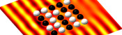
These properties conclude chapter 1 of my thesis. Why not take a break and fill the following diagram with hot liquid before reading on.
)
The results of applying the Calderón projector to two functions. By the properties above, these are (the boundary traces of) a solution of the PDE.
This is the first post in a series of posts about my PhD thesis.
Next post in series
(Click on one of these icons to react to this blog post)
You might also enjoy...


Comments
Comments in green were written by me. Comments in blue were not written by me.
Add a Comment