
Blog
2021-09-25
A few weeks ago, I (virtually) went to Talking Maths in Public (TMiP). TMiP is a conference for anyone involved
in—or interested in getting involved in—any sort of maths outreach, enrichment, or public engagement activity. It was really good, and I highly recommend coming to TMiP 2023.
The Saturday morning at TMiP was filled with a choice of activities, including a puzzle hunt written by me. Each puzzle required the solver to first find a clue hidden in
the conference's Gather-Town-powered virtual Edinburgh (built by the always excellent Katie Steckles), then solve the puzzle to reveal a clue to the final code. Once the final code was found, the solvers could enter
a secret area in the Gather Town space.
The puzzles for the puzzle hunt can be found at mscroggs.co.uk/tmip. For anyone who doesn't have access to the Gather Town space, the numbers that are hidden in the space are:
- Puzzle 1: The mathematician (Thomas Bayes) died in 1761.
- Puzzle 2: The sign claims that Arthur's seat is 1288 links tall.
- Puzzle 3: The sign claims that the maximum capicity of the museum is 2449 people.
- Puzzle 4: Dynamic Earth became a charitable trust in 94.
- Puzzle 5: The 102 bus goes to Dumfries.
The solutions to the five puzzles, and the final puzzle are below. If you want to try the puzzles for yourself, do that now before reading on.
Puzzle 1: The strange shop
A shop has a very strange pricing model. If you buy \(k\) items, then the price (in pence) is decided as follows:
- If \(k\) is prime, then the price is \(k\) pence.
- If \(k\) is not prime, then double \(k\) and add one:
- If the result is prime, that is the price.
- If the result is not prime, keep doubling and adding one until a prime is reached.
You enter the shop with 1761 pence and buy 28 items.
How many pence do you leave the shop with?
Fun fact: If you try to buy 509202 items from the shop, then the shopkeeper cannot work out a price,
as a prime is never reached. It is currently unknown if this is the smallest number of items that
this is true for.
Puzzle 2: The homemade notebook
You make a homemade notebook with 1288 pages:
You take a stack of 1288/4 pieces of paper and fold the entire stack in half so that
each piece of paper makes four pages in the notebook. You number the pages:
you write the number 1 on the front cover, 2 on the inside front cover, and so on
until you write 1288 on the back cover.
While you are looking for your stapler, a strong wind blows the pieces of paper all
over the floor. You pick up one of the pieces of paper and add up the two numbers
you wrote on one side of it.
What is the largest total you could have obtained?
Puzzle 3: The overlapping triangles
You draw three circles that all meet at a point:
You then draw two triangles. The smaller red triangle's vertices are the centres of the circles. The larger blue triangle's vertices are at the points on each circle diametrically opposite the point where all three circles meet:
The area of the smaller red triangle is 2449.
What is the area of the larger blue triangle?
The odd factors
You write down the integers from 94+1 to 2×94 (including 94+1 and 2×94). Under each number, you write down its largest odd factor*.
What is the sum of all the odd factors you have written?
* In this puzzle, factors include 1 and the number itself.
Hint: Doing what the puzzle says may take a long time. Try doing this will some smaller values than 94 first and see if you can spot a shortcut.
The sandwiched quadratic
You know that \(f\) is a quadratic, and so can be written as \(f(x)=ax^2+bx+c\) for some real numbers \(a\), \(b\), and \(c\);
but you've forgetten exactly which quadratic it is. You remember that for all real values of \(x\), \(f\) satisfies
$$\tfrac{1}{4}x^2+2x-8\leqslant f(x)\leqslant(x-2)^2.$$
You also remember that the minimum value of \(f\) is at \(x=0\).
What is f(102)?
The final puzzle
The final puzzle involves using the answers to the five puzzles to find a secret four digit passcode is made up of four non-zero digits. To turn them into clues,
the answers to each puzzle were scored as follows:
Each digit in an answer that is also in the passcode and in the same position in both scores two points; every digit in the answer that is also in the passcode but in a different position scores 1 point. For example, if the passcode was 3317, then:
- 4686 would score 0 points (no digits correct);
- 4676 would score 1 point (7 is a correct digit but in the wrong position);
- 4616 would score 2 points (1 is a correct digit in the correct position);
- 4343 would score 3 points (one of the 3s is a correct digit in the correct position, the other 3 is a correct digit in the wrong position);
- 7333 would score 4 points (one of the 3s is a correct digit in the correct position, the 7 and one of the other 3s are correct digits in wrong positions. Note that the third three scores nothing);
- and 1733 would score 4 points (all four digits are correct digits in wrong positions).
The five clues to the final code are:
- Puzzle 1: 1298 scores 3 points.
- Puzzle 2: 1289 scores 3 points.
- Puzzle 3: 9697 scores 3 points.
- Puzzle 4: 8836 scores 1 point.
- Puzzle 5: 5198 scores 4 points.
(Click on one of these icons to react to this blog post)
You might also enjoy...

Comments
Comments in green were written by me. Comments in blue were not written by me.
⭐ top comment (2021-09-27) ⭐
@Dan: Well spotted, I've edited the postMatthew
Small nitpick on problem 1 fun fact. I think you meant 509202. 509203 is already prime so the price would be 509203. The way you set up the problem (2a_n+1) only gets to (k*2^n-1) if you start with k-1, so your k needs to be one smaller than the Wikipedia's k. ×3 ×3 ×3 ×2 ×2
Dan
Add a Comment
2021-05-22
In this post I'd like to talk about the catchily named Stirling numbers of the second kind, which I first encountered in this Maths Stack Exchange post. I'll start with some motivation for Stirling numbers of the second kind, show how they can be recursively calculated, and then show some interesting features of these numbers.
Suppose a fair die has \(f\) distinct faces, and suppose you roll it \(n\) times. What's the probability that you roll exactly \(k\) distinct faces? Since the die is fair, each sequence of rolls is equally likely, so the probability is given by
$$
\frac{\text{number of ways to roll the die \(n\) times and observe \(k\) distinct faces}}{\text{number of sequences of \(n\) rolls}}.
$$
The number of possible sequences of \(n\) rolls is just \(f^{n}\). And since, if we see exactly \(k\) distinct faces, the \(k\) distinct faces are equally likely to be any of the subsets of size \(k\) out of \(f\). So we have:
$$
\begin{array}{lr}
\text{ways to observe \(k\) distinct faces in \(n\) rolls}\hspace{-7cm}&\\[-7mm]&= (\text{ways to observe \(\{1, 2, \dots, k\}\) in \(n\) rolls}) \times \displaystyle\binom{f}{k}.
\end{array}
$$
Let's think about breaking down the \(n\) rolls into \(k\) subsets based on which rolls matched each face. For example, if \(k = 3\) and the sequence of rolls was \(\{1, 2, 1, 2, 3, 1\}\), then the three subsets would be \(\{1, 3, 6\}, \{2, 4\}\), and \(\{5\}\), where the first subset is \(\{1, 3, 6\}\) because rolls 1, 3, and 6 were face 1. Since each of the \(k\) faces was observed, each subset must be non-empty. Any permutation of these subsets still creates a valid sequence of observations, eg if we swapped the first two subsets then the subsets would correspond to the sequence of rolls \(\{2, 1, 2, 1, 3, 2\}\). And since there are \(k!\) to permute the subsets, we have that the probability is
$$
(\text{ways to partition \(n\) items into \(k\) non-empty subsets}) \times \binom{f}{k} \times k! \times f^{-n}.
$$
The number of ways to partition \(n\) items into \(k\) non-empty subsets is a Stirling number of the second kind, denoted \(\left\{n\atop k\right\}\).
In the same way that the factorial function is technically defined recursively,
$$
x! =
\begin{cases}
1 & \text{if } x = 0,\\
(x - 1)! \thinspace x & \text{if } x > 0,
\end{cases}
$$
we can define the Stirling number of the second kind recursively. If \(n = 0\) and \(k = 0\), then the probability of seeing \(k\) distinct numbers in \(n\) rolls is 1, so we set \(\left\{0\atop 0\right\} = 1\). If \(n \geq 1\) then we are guaranteed to see at least \(1\) distinct face, so \(\left\{n\atop 0\right\} = 0\). If \(n = 0\) and \(k\geq1\), then seeing \(k\) faces is impossible, so \(\left\{0\atop k\right\} = 0\). And if \(k > n\) then seeing \(k\) distinct faces in \(n\) rolls is impossible, so \(\left\{n\atop k\right\} = 0\). These give us the base cases for a recursion. The recursive formula for \(n, k \geq 1\) is given by
$$
\left\{n\atop k\right\} = \left\{n - 1\atop k-1\right\} + k \left\{n - 1\atop k\right\}.
$$
To see why, consider splitting \(n\) items into \(k\) non-empty subsets, and suppose that \(n - 1\) of the items have already been added to subsets. We will consider two cases. In one case, the \(n - 1\) items have only been assigned to \(k - 1\) subsets (making each of these \(k-1\) subsets non-empty) and we are forced to use the \(n\)th item to make the \(k\)th subset non-empty. There are \(\left\{n-1\atop k-1\right\}\) ways that \(n-1\) items can be assigned to make \(k-1\) non-empty subsets, hence the first term in the sum. In the second case, the \(n-1\) items have already been assigned to all \(k\) subsets (making each of the \(k\) subsets non-empty), and we are free to choose which of the \(k\) subsets to put the \(n\)th item in. There are \(\left\{n-1\atop k\right\}\) ways that \(n-1\) items can be assigned to make \(k\) non-empty subsets, and \(k\) choices for the \(n\)th item, hence the second term in the sum.
The plot shows a "Pascal's triangle" for the Stirling numbers of the second kind, which I call "Stirling's second triangle". The top square is \(\left\{0\atop 0\right\}\), the next row contains \(\left\{1\atop 0\right\}, \left\{1\atop 1\right\}\), and so on.
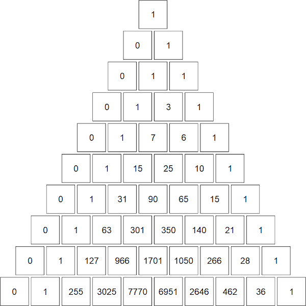
The top ten rows of "Stirling's second triangle"
You can see how the generating rule differs from the one for \(\binom nk\). Instead of
$$
\binom{n}{k} = \binom{n - 1}{k - 1} + \binom{n - 1}{k}
$$
we have our recursive formula. Let's do the 5th row (corresponding to \(n = 4\)) as an example. We know from the base cases that \(\left\{4\atop 0\right\} = 0\). Then \(\left\{4\atop 1\right\} = 0 + 1 \times 1 = 1\), \(\left\{4\atop 2\right\} = 1 + 2 \times 3 = 7\), \(\left\{4\atop 3\right\} = 3 + 3 \times 1 = 6\), and \(\left\{4\atop 4\right\} = 1 + 4 \times 0 = 1\).
)
The diagonal \(\left\{2\atop 2\right\}\), \(\left\{3\atop 2\right\}\), \(\left\{4\atop 2\right\}\), \(\left\{5\atop 2\right\}\), \(\left\{6\atop 2\right\}\), ...
The diagonals in this triangle have some interesting features. Consider the diagonal \(\left\{2\atop 2\right\}\), \(\left\{3\atop 2\right\}\), \(\left\{4\atop 2\right\}\), \(\left\{5\atop 2\right\}\), \(\left\{6\atop 2\right\}\), ... = 1, 3, 7, 15, 31, ... = \(2^1 - 1\), \(2^2 - 1\), \(2^3 - 1\), \(2^4 - 1\), \(2^5 - 1\), ... The triangular numbers 0, 1, 3, 6, 10, 15, ... also make an appearance. I will leave it as an exercise for the reader to show that
$$
\left\{n\atop 2\right\} = 2^{n-1} - 1,$$$$\text{ and } \left\{n\atop n-1\right\} = \binom{n}{2}.
$$
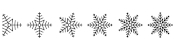
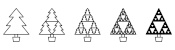
Finally, an interesting feature occurs if you shade in the "Stirling's second triangle" according to the parity of the entry. Let the odd numbers be shaded grey and the white numbers be shaded white. At first it is difficult to discern a pattern, but it a fractal pattern related to the Sierpiński triangle emerges.
)
The top five rows of "Stirling's second triangle" coloured by parity.
)
The top twenty rows of "Stirling's second triangle" coloured by parity.
)
The top thirty rows of "Stirling's second triangle" coloured by parity.
)
The top sixty-six rows of "Stirling's second triangle" coloured by parity.
(Click on one of these icons to react to this blog post)
You might also enjoy...
Comments
Comments in green were written by me. Comments in blue were not written by me.
Add a Comment
2021-01-03
It's 2021, and the Advent calendar has disappeared, so it's time to reveal the answers and annouce the winners.
But first, some good news: with your help, Santa received all his letters and Christmas was saved!
Now that the competition is over, the questions and all the answers can be found here.
Before announcing the winners, I'm going to go through some of my favourite puzzles from the calendar, reveal the solution and a couple of other interesting bits and pieces.
Highlights
My first highlight is this puzzle from 5 December, that I think doesn't seem obvious that there's even a unique answer until you spot some nice properties of
dice.
5 December
Carol rolled a large handful of six-sided dice. The total of all the numbers Carol got was 521. After some calculating, Carol worked out that the probability that of her total being 521
was the same as the probability that her total being 200. How many dice did Carol roll?
My next highlight is the puzzle from 15 December. I had a lot of fun trying to write this one. At the end, I tell you that T represents 4: this puzzle still has a unique answer without this,
but it was too hard to get started.
15 December
When talking to someone about this Advent calendar, you told them that the combination of XMAS and MATHS is GREAT.
They were American, so asked you if the combination of XMAS and MATH is great; you said SURE. You asked them their name; they said SAM.
Each of the letters E, X, M, A, T, H, S, R, U, and G stands for a different digit 0 to 9. The following sums are correct:
|
| ||||||||||||||||||||||||||||||||||
Today's number is SAM. To help you get started, the letter T represents 4.
My next highlight is the puzzle from 16 December. I had a lot of fun writing this one too. At least a few people seem to have enjoyed solving it,
as indicated by this comment.
16 December
Solve the crossnumber to find today's number. No number starts with 0.
|
| |||||||||||||||||||||||||||||||||
My final highlight is the puzzle from 21 December. My method for solving this one was quite complicated. Let me know in the comments or on Twitter if you have a better way of solving it.
21 December
There are 3 ways to order the numbers 1 to 3 so that no number immediately follows the number one less that itself:
- 3, 2, 1
- 1, 3, 2
- 2, 1, 3
Today's number is the number of ways to order the numbers 1 to 6 so that no number immediately follows the number one less that itself.
Hardest and easiest puzzles
Once you've entered 24 answers, the calendar checks these and tells you how many are correct. I logged the answers that were sent
for checking and have looked at these to see which puzzles were the most and least commonly incorrect. The bar chart below shows the total number
of incorrect attempts at each question.
| 1 | 2 | 3 | 4 | 5 | 6 | 7 | 8 | 9 | 10 | 11 | 12 | 13 | 14 | 15 | 16 | 17 | 18 | 19 | 20 | 21 | 22 | 23 | 24 |
| Day | |||||||||||||||||||||||
You can see that the most difficult puzzles were those on
6,
14,
19,
21, and
24 December;
and the easiest puzzles were on
3,
9,
10,
16, and
17 December.
The solutions
The solutions to all the individual puzzles can be found here. If you want to read some alternative solutions to the puzzles, you can find Alira's solutions here, including a very nice explanation of how the final clues fit together to find the directions to Santa's house.
Using the daily clues, it was possible to work out that Santa's house could be found by following the directions 3,7,1,1,4,3,3,4,9,3,3,9 on this map.
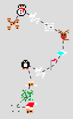
Directions to Santa's house.
Due to the way the Advent compass worked, there are actually a few different ways to get to Santa's house. For example, 7,5,7,1,1,4,3,3,4,9,3,3 also gets you there:
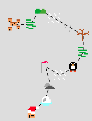
Alternative directions to Santa's house.
I'll leave you to work out how many different ways there are to get there...
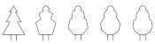
Here's the full collection of tiles that you could find by walking around the map:
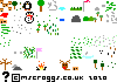
The map tiles.
The winners
And finally (and maybe most importantly), on to the winners: 223 people found Santa's house entered the competition. This is quite a lot more than in previous years:
| 2015 | 2016 | 2017 | 2018 | 2019 | 2020 |
| Year | |||||
From the correct answers, the following 10 winners were selected:
| 1 | Mars He |
| 2 | Ben Baker |
| 3 | Amelia Taylor |
| 4 | Alex Ayres |
| 5 | Hannah Charman |
| 6 | Diane Keimel |
| 7 | Alex Burlton |
| 8 | Rob March |
| 9 | Mahmood Hikmet |
| 10 | Guillermo Heras Prieto |
Congratulations! Your prizes will be on their way shortly.
The prizes this year include 2020 Advent calendar T-shirts. If you didn't win one, but would like one of these, I've made them available to buy at merch.mscroggs.co.uk alongside the T-shirts from previous years.
Additionally, well done to
4nder, Ashley Frazer Jarvis, Aaron Stiff, Alan Buck, Alejandro Villarreal, Alex Bolton, Alex Davis, Alex Klapheke, Alexander Rakitin, Anders Kaseorg, Andrew, Andrew P Turner, Andy Ennaco, Annabel, Anthony Della Pella, Artie Smith, Athena, Austin, Austin Shapiro, Beau Ferguson, Becky Russell, Ben Buchwald, Ben Jones, Ben Reiniger, Benjamin Tozer, Bennet, Beth Jensen, Blake, Brennan Dolson, Brian Carnes, Brian Wellington, Burak Kadron, Caleb Likely, Callum Hobbis, Carl Westerlund, Carmen Günther, Cath Simpson, Cathy Hooper, Chris Hellings, Christy Hales, Colin, Colin Brockley, Connie, Corbin Groothuis, Cory Peters, Cosmo Viola, Dan Colestock, Dan DiMillo, Dan McIntyre, Dan Whitman, Dana Sussman, Daniel De la Paz, David, David Ault, David Berardo, David Fox, David Kendel, David Mitchell, David Parmenter, David and Ivy Walbert, Dean Thomas, Deborah Tayler, Don Anderson, Donagh Collins, Elizabeth Blackwell, Emilie Heidenreich, Emily Troyer, Eric Kolbusz, Eric Skoglund, Erik Eklund, Eva, Evan Louis Robinson, Fionn Woodcock, Frances Haigh, Frank Kasell, Franklin Ta, Fred Verheul, Georges, Gabriella Pinter, Gert-Jan de Vries, Graham Greve, Gregory Loges, Gwendal Collet, Harry Allen, Heerpal Sahota, Helen, Helen Matthews, Herschel Pecker, Håkon Balteskard, Ivan Arribas, Jacob Young, James Demers, James Laver, Jan, Jason Demers, Jason Kass, Jean-Sébastien Turcotte, Jeff Rubin, Jefff Michael, Jen Huang, Jessica Marsh, Jim Rogers, Joe Gage, Johan Asplund, John Alasdair Warwicker, Jon Foster, Jon Lipscombe, Jon Palin, Jonathan Chaffer, Jonathan Forsythe, Jonathan Winfield, Jordan Susskind, Jorge del Castillo, Kai Lam, Karen Climis, Keith Pound, Ken Cheung, Killeen, Kristen Koenigs, Kristin Gramza, Kurt Engleman, Laura Midgley, Lauren Woolsey, Lewis Dyer, Linus Banghart-Linn, Liz Madisetti, Louis de Mendonca, Magnus Eklund, Mark Stambaugh, Martijn O., Martin Harris, Martin Holtham, Martine Nome, Matt Askins, Matt Hutton, Matthew Reynier, Matthew Riggle, Matthew Schulz, Matthew Scroggs, Matthias Planitzer, Maxime Rivet, Maximilian Pfister, Michael DeLyser, Michael Prescott, Mihai Zsisku, Mike Hands, Moritz Stocker, Nadine Chaurand, Nathan Chun, Nick C, Nick Keith, Nick Mohr, Norvin Richards, Olov Wilander, Pamela Docherty, Pau Batlle, Paul Livesey, Pranshu Gaba, Ray Arndorfer, Rea, Reuben Cheung, Riccardo Lani, Richard Pemberton, Rileigh Luczak, Road White, Roni, Rosie Paterson, Russ Collins, Ruth Franklin, Ryan Coomer, Ryan Seldon, Ryan Wise, Sam Dreilinger, Sam Hartburn, Sammie Buzzard, Sara Van Hoy, Sarah Brook, Saul Freedman, Scott, Sean, Sean Carmody, Sean Henderson, Sean McDonald, Sebastian, Selina Glauert, Seth Cohen, Shivanshi Adlakha, Simon Schneider, Sophie Maclean, Spencer B., Stephen Cappella, Stephen Dainty, Stephen Jasina, Steve Blay, Steve Paget, Steven Richardson, Susana Early, Tarim, Tim Holman-Wilkens, Tim Lewis, Todd Geldon, Tom Fryers, Tony Mann, Tristan Shephard, Valentin Valciu, Vinesh, Yasha, Yuliya Nesterova, Yurie Ito, and Zachary Polansky
who all also found Santa's house but were too unlucky to win prizes this time.
See you all next December, when the Advent calendar will return.
(Click on one of these icons to react to this blog post)
You might also enjoy...


Comments
Comments in green were written by me. Comments in blue were not written by me.
Dec 15th was my favorite. I kept making a logical error and had to restart, so it took me way to long, but I really enjoyed it.
The 16th was just cheeky, after I spent way to much time on the 15th it was nice to have something like that!
It's been 16+ years since I did any probability or combinations and permutations, so it was nice to brush off that part of my brain, not that I did any of them well, but it should serve me well when my kids start doing them and ask me for help.×4 ×3 ×3 ×3 ×3
The 16th was just cheeky, after I spent way to much time on the 15th it was nice to have something like that!
It's been 16+ years since I did any probability or combinations and permutations, so it was nice to brush off that part of my brain, not that I did any of them well, but it should serve me well when my kids start doing them and ask me for help.
Dave
You can solve the Dec 21 puzzle using the principle of inclusion/exclusion:
-There are 6! total ways of arranging 6 numbers.
-Now we have to exclude the ones that don't fit. How many ways have 2 following 1? You can think of 12 as a pair, so you're arranging 12/3/4/5/6 in any order, so there are 5! ways to do this. And there are (5 choose 1)=5 total pairs that might exist, so there are 5*5! ways that have either 12, 23, 34, 45, or 56.
-Of course, we've double counted some that have more than one pair. (This is where inclusion/exclusion comes in, we have to include them back in). So how many have, say, 12 and 45? Well now we're arranging 12/3/45/6, so there are 4! ways to do so. There are (5 choose 2)=10 different pairs, so the double counting was 10*4!.
-We continue this on, and inclusion/exclusion says we keep alternating adding and subtracting as we add more pairs, so the answer is:
6!
- (5 choose 1) * 5!
+ (5 choose 2) * 4!
- (5 choose 3) * 3!
+ (5 choose 4) * 2!
- (5 choose 5) * 1!
= 309×6 ×4 ×3 ×3 ×3
-There are 6! total ways of arranging 6 numbers.
-Now we have to exclude the ones that don't fit. How many ways have 2 following 1? You can think of 12 as a pair, so you're arranging 12/3/4/5/6 in any order, so there are 5! ways to do this. And there are (5 choose 1)=5 total pairs that might exist, so there are 5*5! ways that have either 12, 23, 34, 45, or 56.
-Of course, we've double counted some that have more than one pair. (This is where inclusion/exclusion comes in, we have to include them back in). So how many have, say, 12 and 45? Well now we're arranging 12/3/45/6, so there are 4! ways to do so. There are (5 choose 2)=10 different pairs, so the double counting was 10*4!.
-We continue this on, and inclusion/exclusion says we keep alternating adding and subtracting as we add more pairs, so the answer is:
6!
- (5 choose 1) * 5!
+ (5 choose 2) * 4!
- (5 choose 3) * 3!
+ (5 choose 4) * 2!
- (5 choose 5) * 1!
= 309
Todd
Add a Comment
2020-12-03
In November, I spent some time designing this year's Chalkdust puzzle Christmas card.
)
The card looks boring at first glance, but contains 9 puzzles. By splitting the answers into two digit numbers, then colouring the regions labelled with each number (eg if an answer to a question in the red section is 201304, colour the regions labelled 20, 13 and 4 red), you will reveal a Christmas themed picture.
If you want to try the card yourself, you can download this pdf. Alternatively, you can find the puzzles below and type the answers in the boxes. The answers will be automatically be split into two digit numbers, and the regions will be coloured...
Grey/black | ||
| 1. | How many odd numbers can you make (by writing digits next to each other, so 13, 1253, and 457 all count) using the digits 1, 2, 3, 4, 5, and 7 each at most once (and no other digits)? | Answer |
| 2. | Carol made a book by stacking 40300 pieces of paper, folding the stack in half, then writing the numbers 1 to 161200 on the pages. She then pulled out one piece of paper and added up the four numbers written on it. What is the largest number she could have reached? | Answer |
| 3. | What is the sum of all the odd numbers between 0 and 130376? | Answer |
White/yellow | ||
| 4. | There are three cards with integers written on them. The pairs of cards add to 31, 35 and 36. What is the sum of all three cards? | Answer |
| 5. | What is the volume of the smallest cuboid that a square-based pyramid with volume 1337 can fit inside?? | Answer |
| 6. | What is the lowest common multiple of 305 and 671? | Answer |
Red | ||
| 7. | Holly rolled a huge pile of dice and added up all the top faces to get 6136. She realised that the probability of getting 6136 was the same as getting 9999. How many dice did she roll? | Answer |
| 8. | How many squares (of any size) are there in a 14×16 grid of squares? | Answer |
| 9. | Ivy picked a number, removed a digit, then added her two numbers to get 155667. What was her original number? | Answer |
(Click on one of these icons to react to this blog post)
You might also enjoy...
Comments
Comments in green were written by me. Comments in blue were not written by me.
@JDev: lots of the card will still be brown once you're done, but you should see a nice picture. Perhaps one of your answers is wrong, making a mess of the picture? ×1 ×1 ×1 ×1
Matthew
I finished all of the puzzles but the picture is far from colored in. Am I missing something?
These puzzles have been a blast!×1 ×1 ×1 ×1
These puzzles have been a blast!
JDev
@Tara: I initially made the same mistake. Maybe you didn't take into account that 6 is not one of the available digits in question 1?×1 ×2
Sean
@Tara: Yes, looks like you may have got an incorrect answer for one of the black puzzles ×1 ×2 ×1 ×1 ×1
Matthew
Add a Comment
2020-11-22
This year, the front page of mscroggs.co.uk will once again feature an Advent calendar, just like
in the five previous Decembers.
Behind each door, there will be a puzzle with a three digit solution. The solution to each day's puzzle forms part of a logic puzzle:
It's nearly Christmas and something terrible has happened: you've just landed in a town in the Arctic circle with a massive bag of letters for Santa, but you've lost to instructions for how to get to Santa's house near the north pole. You need to work out where he lives and deliver the letters to him before Christmas is ruined for everyone.
Due to magnetic compasses being hard to use near the north pole, you brought with you a special Advent compass. This compass has nine numbered directions. Santa has given the residents of the town clues about a sequence of directions that will lead to his house; but in order to keep his location secret from present thieves, he gave each resident two clues: one clue is true, and one clue is false.
The residents' clues will reveal to you a seqeunce of compass directions to follow. You can try out your sequences on this map.
Behind each day (except Christmas Day), there is a puzzle with a three-digit answer. Each of these answers forms part of a resident's clue. You must use these clues to work out how to find Santa's house.
Ten randomly selected people who solve all the puzzles, find Santa's house, and fill in the entry form behind the door on the 25th will win prizes!
)
The winners will be randomly chosen from all those who submit the entry form before the end of 2020. Each day's puzzle (and the entry form on Christmas Day) will be available from 5:00am GMT. But as the winners will be selected randomly,
there's no need to get up at 5am on Christmas Day to enter!
As you solve the puzzles, your answers will be stored. To share your stored answers between multiple devices, enter your email address below the calendar and you will be emailed a magic link to visit on your other devices.
To win a prize, you must submit your entry before the end of 2020. Only one entry will be accepted per person. If you have any questions, ask them in the comments below or on Twitter.
So once December is here, get solving! Good luck and have a very merry Christmas!
(Click on one of these icons to react to this blog post)
You might also enjoy...
Comments
Comments in green were written by me. Comments in blue were not written by me.
Nice one today (16 December) :)
Did he?... did he really?... starts to look like it... yes he did! :D×3 ×6 ×3 ×1 ×2
Did he?... did he really?... starts to look like it... yes he did! :D
Gert-Jan
@Dean: you can also go through each answer one at a time and change a digit; if the number of wrong answers goes up then your answer for that question was correct×1 ×1
A
@Dean: Yes, I'm planning to change how that bit works. Check back tomorrow or the next day for a more fun finish! ×1
Matthew
A bit harsh that we can’t tell exactly which answers are wrong! I won’t have time to revisit every puzzle - and its kind of less fun redoing something that is already correct... :-(
Dean
Add a Comment