
Blog
2013-12-23
Here is a collection of Christmas relates mathematical activities.
Flexagons
I first encountered flexagons sometime around October 2012. Soon after, we used this template to make them at school with year 11 classes who had just taken GCSE papers as a fun but mathematical activity. The students loved them. This lead me to adapt the template for Christmas:
)
And here is an uncoloured version of the template on that site if you'd like to colour it yourself and a blank one if you'd like to make your own patterns:
)
The excitement of flexagons does not end there. There are templates around for six faced flexagons and while writing this piece, I found this page with templates for a great number of flexagons. In addition, there is a fantastic article by Martin Gardner and a two part video by Vi Hart.
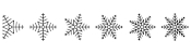
Fröbel stars
I discovered the Fröbel star while searching for a picture to be the Wikipedia Maths Portal picture of the month for December 2013. I quickly found these very good instructions for making the star, although it proved very fiddly to make with paper I had cut myself. I bought some 5mm quilling paper which made their construction much easier. With a piece of thread through the middle, Fröbel starts make brilliant tree decorations.
(Click on one of these icons to react to this blog post)
You might also enjoy...


Comments
Comments in green were written by me. Comments in blue were not written by me.
Add a Comment
2013-12-15
Last week, I was watching Pointless and began wondering how likely it is that a show features four new teams.
On the show, teams are given two chances to get to the final—if they are knocked out before the final round on their first appearance, then they return the following episode. In all the following, I assumed that there was an equal chance of all teams winning.
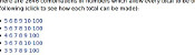
If there are four new teams on a episode, then one of these will win and not return and the other three will return. Therefore the next episode will have one new team (with probability 1). If there are three new teams on an episode: one of the new teams could win, meaning two teams return and two new teams on the next episode (with probability 3/4); or the returning team could win, meaning that there would only one new team on the next episode. These probabilities, and those for other numbers of teams are shown in the table below:
| No of new teams today | |||||
Noof new teams tomorrow
| 1 | 2 | 3 | 4 | |
| 1 | 0 | 0 | \(\frac{1}{4}\) | 1 | |
| 2 | 0 | \(\frac{1}{2}\) | \(\frac{3}{4}\) | 0 | |
| 3 | \(\frac{3}{4}\) | \(\frac{1}{2}\) | 0 | 0 | |
| 4 | \(\frac{1}{4}\) | 0 | 0 | 0 | |
Call the probability of an episode having one, two, three or four new teams \(P_1\), \(P_2\), \(P_3\) and \(P_4\) respectively. After a few episodes, the following must be satisfied:
$$P_1=\frac{1}{4}P_3+P_4$$
$$P_2=\frac{1}{2}P_2+\frac{3}{4}P_3$$
$$P_3=\frac{3}{4}P_3+\frac{1}{2}P_4$$
$$P_4=\frac{1}{4}P_1$$
And the total probability must be one:
$$P_1+P_2+P_3+P_4=1$$
These simultaneous equations can be solved to find that:
$$P_1=\frac{4}{35}$$
$$P_2=\frac{18}{35}$$
$$P_3=\frac{12}{35}$$
$$P_4=\frac{1}{35}$$
So the probability that all the teams on an episode of Pointless are new is one in 35, meaning that once in every 35 episodes we should expect to see all new teams.
Edit: This blog answered the same question in a slightly different way before I got here.
(Click on one of these icons to react to this blog post)
You might also enjoy...

Comments
Comments in green were written by me. Comments in blue were not written by me.
Add a Comment
2013-07-24
A news story on the BBC Website caught my eye this morning. It reported the following "uncanny coincidence" between a Northern Irish baby and a Royal baby:

But both new mothers share the name Catherine, the same birthday - 9 January - and now their sons also share the same birth date.

I decided to work out just how uncanny this is.
The Office for National Statistics states that 729,674 babies are born every year in the UK. This works out at 1,999 babies born each day, assuming that births are uniformly distributed, so there will be approximately 1,998 babies who share Price Nameless's birthday.
So, what is the chance of the mother of one of these babies having the same birthday as Princess Kate? To work this out I used a method similar to that which is used in the birthday "paradox", which tells us that in a group of 23 people there is a more than 50% chance of two people sharing a birthday, but that's another story.
First, we look at one of our 1,998 mothers. The chance that she shares Princess Kate's birthday is 1/365 (ignoring leap days). The chance that she does not share Princess Kate's Birthday is 364/365.
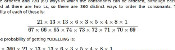
Next we work out the probability that none of our 1,998 mothers shares Princess Kate's birthday. As our mothers' birthdays are independent we can multiply the probabilities together to do this (this is why we are looking at the probability of not sharing a birthday instead of sharing a birthday). Our probability therefore is \(\left(\frac{364}{365}\right)^{1998} = 0.00416314317\).
Back to the original question, we wanted to know the probability that one of our mothers shares Princess Kate's birthday. To calculate this we do take 0.00416314317 away from 1. This gives 0.99583685682 or 99.6%.
There is a 99.6% chance that there is a resident of the UK who shares the same birthday as Princess Kate and had a child on the same day.
Uncanny.
But let's be fair. The mother in our story is also called Kate. So what are the chances of that? In fact, the same method can be followed, working with the probability of having neither the same birthday or name as Princess Kate.
I think it is safe to assume that this would still be considered news-worthy if our non-princess was called Katie, Cate, Cathryn, Katie-Rose or any other name which is commonly shortened to Kate, so I included a number of variations and used this fantastic tool to find the probability of a mother being called Kate. The data only goes back to 1996, but as the name is dropping in popularity, we can assume that before 1996 at least 1.5% of babies were called Kate. Disregarding males, we can estimate that 3% of mothers are called Kate.
If anyone would like the details of the rest of the calculation, please comment on this post and I will include it here. For anyone who trusts me and isn't curious, I eventually found that the probability of none of our 1,998 mothers share the same name and birthday as Princess Kate is 0.84855028964. So the probability of another Kate having a child on the same day and sharing Princess Kate's birthday is 0.15144971035 or 15.1%. Just over one in seven.
So this is as uncanny as anything else which has a probability of one in seven, such as the Royal baby being born on a Monday (uncanny!).
(Click on one of these icons to react to this blog post)
You might also enjoy...


Comments
Comments in green were written by me. Comments in blue were not written by me.
Add a Comment
2013-07-11
On 19 June, the USB temperature sensor I ordered from Amazon arrived. This sensor is now hooked up to my Raspberry Pi, which is taking the temperature every 10 minutes, drawing graphs, then uploading them here. Here is a brief outline of how I set this up:
Reading the temperature
I found this code and adapted it to write the date, time and temperature to a text file. I then set cron to run this every 10 minutes. It writes the data to a text file (/var/www/temperature2) in this format:
2013 06 20 03 50,16.445019
2013 06 20 04 00,16.187843
2013 06 20 04 10,16.187843
2013 06 20 04 20,16.187843
2013 06 20 04 00,16.187843
2013 06 20 04 10,16.187843
2013 06 20 04 20,16.187843
Plotting the graphs
I found a guide somewhere on the internet about how to draw graphs with Python using Pylab/Matplotlib. If you have any idea where this could be, comment below and I'll put a link here.
In the end my code looked like this:
python
import timeimport matplotlib as mpl
mpl.use("Agg")
import matplotlib.pylab as plt
import matplotlib.dates as mdates
ts = time.time()
import datetime
now = datetime.datetime.fromtimestamp(ts)
st = mdates.date2num(datetime.datetime(int(float(now.strftime("%Y"))),
int(float(now.strftime("%m"))),
int(float(now.strftime("%d"))),
0, 0, 0))
weekst = st - int(float(datetime.datetime.fromtimestamp(ts).strftime("%w")))
f = file("/var/www/temperature2","r")
t = []
s = []
tt = []
ss = []
u = []
v = []
g = []
h = []
i = []
weekt = []
weektt = []
weeks = []
weekss = []
mini = 1000
maxi = 0
cur = -1
datC = 0
for line in f:
fL = line.split(",")
fL[0] = fL[0].split(" ")
if cur == -1:
cur = mdates.date2num(datetime.datetime(int(float(fL[0][0])),
int(float(fL[0][1])),
int(float(fL[0][2])),
0,0,0))
datC = mdates.date2num(datetime.datetime(int(float(fL[0][0])),
int(float(fL[0][1])),
int(float(fL[0][2])),
int(float(fL[0][3])),
int(float(fL[0][4])),
0))
u.append(datC)
v.append(fL[1])
if datC >= st and datC <= st + 1:
t.append(datC)
s.append(fL[1])
if datC >= st - 1 and datC <= st:
tt.append(datC + 1)
ss.append(fL[1])
if datC >= weekst and datC <= weekst + 7:
weekt.append(datC)
weeks.append(fL[1])
if datC >= weekst - 7 and datC <= weekst:
weektt.append(datC + 7)
weekss.append(fL[1])
if datC > cur + 1:
g.append(cur)
h.append(mini)
i.append(maxi)
mini = 1000
maxi = 0
cur = mdates.date2num(datetime.datetime(int(float(fL[0][0])),
int(float(fL[0][1])),
int(float(fL[0][2])),
0,0,0))
mini = min(float(fL[1]),mini)
maxi = max(float(fL[1]),maxi)
g.append(cur)
h.append(mini)
i.append(maxi)
plt.plot_date(x=t,y=s,fmt="r-")
plt.plot_date(x=tt,y=ss,fmt="g-")
plt.xlabel("Time")
plt.ylabel("Temperature (#^\circ#C)")
plt.title("Daily")
plt.legend(["today","yesterday"], loc="upper left",prop={"size":8})
plt.grid(True)
plt.gca().xaxis.set_major_formatter(mdates.DateFormatter("%H:%M"))
plt.gcf().subplots_adjust(bottom=0.15,right=0.99)
labels = plt.gca().get_xticklabels()
plt.setp(labels,rotation=90,fontsize=10)
plt.xlim(st,st + 1)
plt.savefig("/var/www/tempr/tg1p.png")
plt.clf()
plt.plot_date(x=weekt,y=weeks,fmt="r-")
plt.plot_date(x=weektt,y=weekss,fmt="g-")
plt.xlabel("Day")
plt.ylabel("Temperature (#^\circ#C)")
plt.title("Weekly")
plt.legend(["this week","last week"], loc="upper left",prop={"size":8})
plt.grid(True)
plt.gca().xaxis.set_major_formatter(mdates.DateFormatter(" %A"))
plt.gcf().subplots_adjust(bottom=0.15,right=0.99)
labels = plt.gca().get_xticklabels()
plt.setp(labels,rotation=0,fontsize=10)
plt.xlim(weekst,weekst + 7)
plt.savefig("/var/www/tempr/tg2p.png")
plt.clf()
plt.plot_date(x=u,y=v,fmt="r-")
plt.xlabel("Date & Time")
plt.ylabel("Temperature (#^\circ#C)")
plt.title("Forever")
plt.grid(True)
plt.gca().xaxis.set_major_formatter(mdates.DateFormatter("%d/%m/%y %H:%M"))
plt.gcf().subplots_adjust(bottom=0.25,right=0.99)
labels = plt.gca().get_xticklabels()
plt.setp(labels,rotation=90,fontsize=8)
plt.savefig("/var/www/tempr/tg4p.png")
plt.clf()
plt.plot_date(x=g,y=h,fmt="b-")
plt.plot_date(x=g,y=i,fmt="r-")
plt.xlabel("Date")
plt.ylabel("Temperature (#^\circ#C)")
plt.title("Forever")
plt.legend(["minimum","maximum"], loc="upper left",prop={"size":8})
plt.grid(True)
plt.gca().xaxis.set_major_formatter(mdates.DateFormatter("%d %b"))
plt.gcf().subplots_adjust(bottom=0.15,right=0.99)
labels = plt.gca().get_xticklabels()
plt.setp(labels,rotation=90,fontsize=8)
plt.savefig("/var/www/tempr/tg3p.png")
If there's anything in there you don't understand, comment below and I'll try to fill in the gaps.
Uploading the graphs
Finally, I upload the graphs to mscroggs.co.uk/weather.
To do this, I set up pre-shared keys on the Raspberry Pi and this server and added
the following as a cron job:
bash
0 * * * * scp /var/www/tempr/tg*p.png username@mscroggs.co.uk:/path/to/folder
I hope this was vaguely interesting/useful. I'll try to add more details and updates over time. If you are building something similar, please let me know in the comments; I'd love to see what everyone else is up to.
Edit: Updated to reflect graphs now appearing on mscroggs.co.uk not catsindrag.co.uk.
(Click on one of these icons to react to this blog post)
You might also enjoy...


Comments
Comments in green were written by me. Comments in blue were not written by me.
Add a Comment
2012-11-02
This is the second post in a series of posts about tube map folding.
Following my previous post, I did a little more folding.
The post was linked to on Going Underground's Blog where it received this comment:
)
In response to which I made this from 48 tube maps:
)
Also since the last post, I left 49 tetrahedrons at tube stations in a period of just over two weeks. Here's a pie chart showing which stations I left them at:
)
Of these 49, only three were still there the next time I passed through the station:
)
Due to the very low recapture rate, little more analysis can be done. Although I do wonder where they all ended up. Do you work at one of those stations and threw some away? Or did you pass through a station and pick one up? Or was it aliens and ghosts?
For my next trick, I want to gather a team of people, pick a day, and leave one at every station that day. If you want to join me, comment on this post, tweet me or comment on reddit and we can formulate a plan. Including your nearest station(s) in your message will help us sort out who takes which stations...
Previous post in series

This is the second post in a series of posts about tube map folding.
Next post in series

(Click on one of these icons to react to this blog post)
You might also enjoy...


Comments
Comments in green were written by me. Comments in blue were not written by me.
Add a Comment